
Euler's Eyes
2026-10-30
The central limit theorem
Roll one die: each face has the same chance, and the graph of the probabilities is flat. Roll two and add: the sum 7 is the most likely, and the graph becomes a triangle. Roll ten, thirty, a hundred: the graph of the sum gradually takes the shape of a bell. The same happens if, instead of dice, we add coins, roulette wheels or measurement errors. This surprising fact is the central limit theorem.
De Moivre and Laplace
In 1733 Abraham de Moivre showed the phenomenon for coins: the number of heads in many tosses has a distribution close to the curve $e^{-x^2}$. Laplace extended the result, in a work of 1810, to sums of arbitrary chances, as long as they are independent and none of them dominates the others.
In modern language: let $X_1, X_2, \ldots, X_n$ be independent chances, all with the same distribution, with mean $\mu$ and variance $\sigma^2$. The sum $S_n = X_1 + \cdots + X_n$ has mean $n\mu$ and standard deviation $\sigma\sqrt{n}$, and
$$\frac{S_n - n\mu}{\sigma\sqrt{n}}$$has, when $n$ is large, a distribution ever closer to the standard normal, with density $\frac{1}{\sqrt{2\pi}}e^{-x^2/2}$.
The dice
For one die, $\mu = 3.5$ and
$$\sigma^2 = \frac{1^2 + 2^2 + \cdots + 6^2}{6} - 3.5^2 = \frac{91}{6} - \frac{49}{4} = \frac{35}{12}.$$The sum of $n$ dice has mean $3.5\,n$ and standard deviation $\sqrt{\frac{35n}{12}}$. The figure compares the exact distribution of the sum with the normal curve of the same mean and standard deviation. Move the slider and see how, already with a few dice, the two almost coincide:
With 100 dice, the mean is 350 and the standard deviation is $\sqrt{\frac{3500}{12}} \approx 17.1$. The chance that the sum falls between 330 and 370, about 1.2 standard deviations on each side, is roughly 76%. Nobody needs to count the $6^{100}$ possible combinations.
Why errors are normal
Laplace saw in the theorem the explanation of a fact of astronomy. Every measurement has an error, and the error is the sum of many small causes: the trembling of the instrument, the air, the observer’s eye, the temperature. If each cause contributes a little and independently, the theorem says that the total error follows the normal curve, whatever the distribution of each cause. In 1809 Gauss had justified the method of least squares by assuming normal errors; Laplace’s theorem, the next year, gave a reason for that assumption.
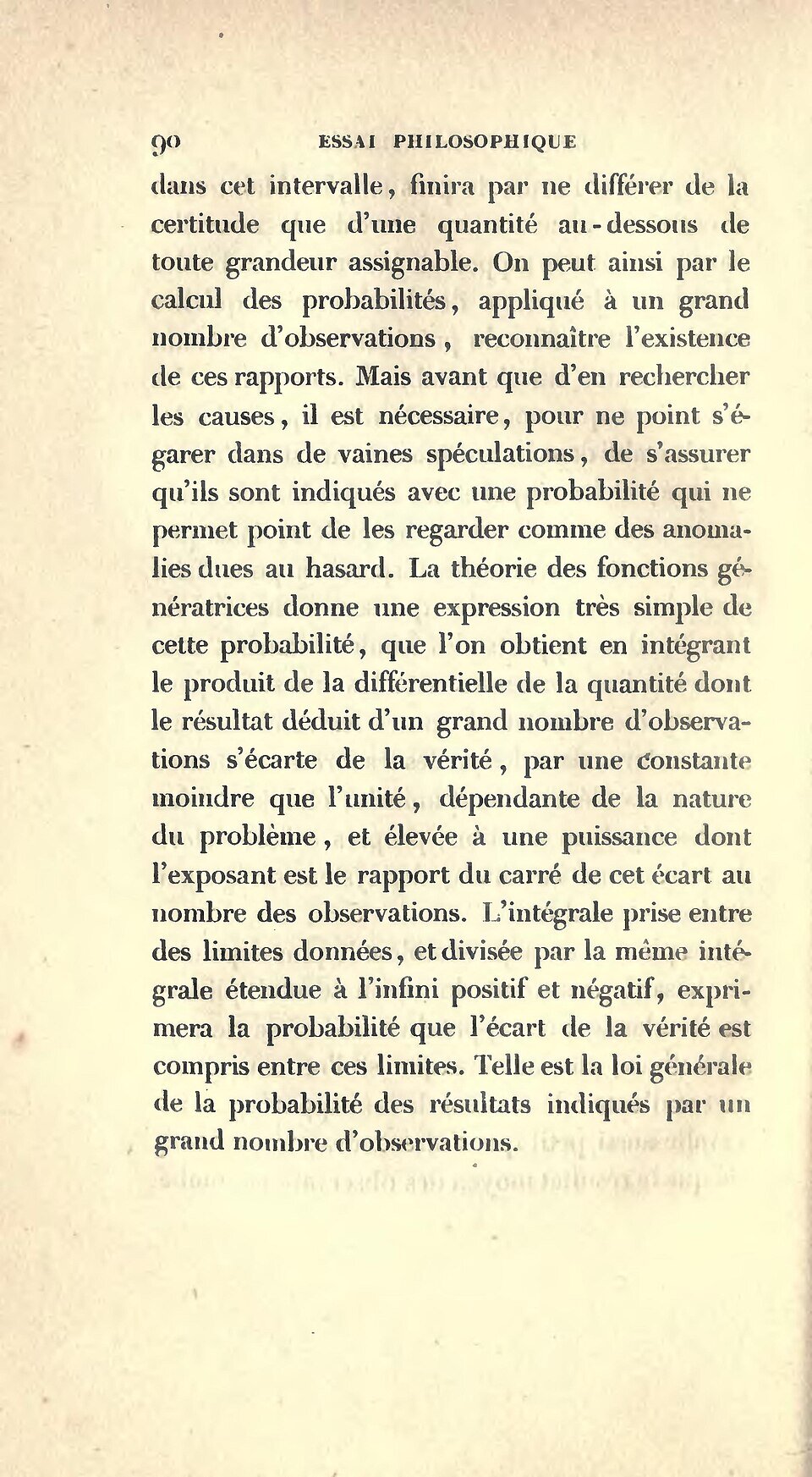
In the proof, Laplace used a new tool: instead of working with the probabilities, he worked with a transform of them, what is today called the characteristic function. The transform of an independent sum is the product of the transforms, and products are easier to control than sums. Laplace’s proof did not have today’s rigour; the exact conditions were established by Aleksandr Lyapunov in 1901 and Jarl Lindeberg in 1922.
Exercise: a hundred coins
We toss 100 fair coins. Use the central limit theorem to estimate the chance that the number of heads falls between 40 and 60.
Each coin counts 1 (heads) or 0 (tails), with $\mu = \frac{1}{2}$ and $\sigma^2 = \frac{1}{4}$. The sum has mean 50 and standard deviation $\sqrt{100 \cdot \frac{1}{4}} = 5$. The interval from 40 to 60 goes from $-2$ to $+2$ standard deviations, and the normal gives about 95% in that interval. The exact value, counting combinations, is 96.5%; the difference shrinks if we use the interval from 39.5 to 60.5, which accounts for the sum taking only integer values.
Exercise: the mean of many measurements
An instrument measures a length with an error of standard deviation 2 mm. What is the standard deviation of the mean of 25 independent measurements?
The sum of the 25 measurements has standard deviation $2\sqrt{25} = 10$ mm. The mean is the sum divided by 25, and so is its deviation: $\frac{10}{25} = 0.4$ mm. In general, the mean of $n$ measurements has deviation $\frac{\sigma}{\sqrt{n}}$: to gain one decimal place of precision, one must measure a hundred times more.
Sources: Pierre-Simon Laplace, “Mémoire sur les approximations des formules qui sont fonctions de très grands nombres et sur leur application aux probabilités”, Mémoires de la classe des sciences mathématiques et physiques de l’Institut (1809, published 1810) · Abraham de Moivre, Approximatio ad summam terminorum binomii (a+b)ⁿ in seriem expansi (1733) · George Pólya, “Über den zentralen Grenzwertsatz der Wahrscheinlichkeitsrechnung und das Momentenproblem”, Mathematische Zeitschrift 8 (1920) · Hans Fischer, A History of the Central Limit Theorem (2011).
All topics on Pierre-Simon Laplace · ← Classical probability and the Gaussian integral · Will the Sun rise tomorrow? The rule of succession →