
Euler's Eyes
2026-10-14
Maxwell's equations: from Faraday's lines of force to vectors
I was at first almost frightened when I saw such mathematical force made to bear upon the subject, and then wondered to see that the subject stood it so well.
— Michael Faraday, letter to Maxwell (25 March 1857)
Until 1820, electricity and magnetism were separate subjects. Electricity made sparks and raised the hair on your head; magnetism made compasses point north. That year, during a lecture at the University of Copenhagen, the Dane Hans Christian Oersted connected a battery to a wire and saw a nearby magnetic needle move. Electric current produced magnetism.
Faraday’s lines of force
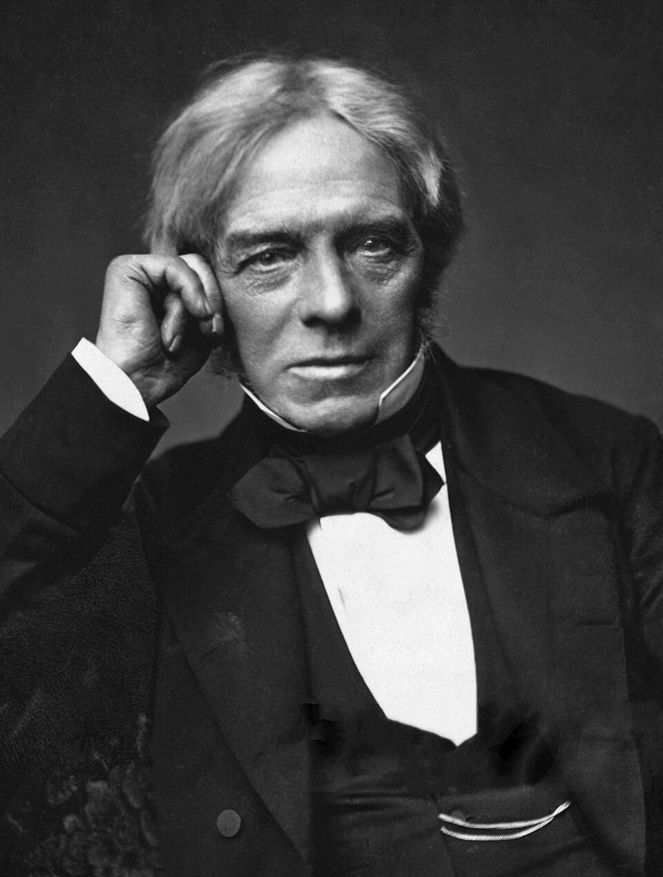
In London, Michael Faraday, a blacksmith’s son who had left school at 13 to become a bookbinder’s apprentice, took the discovery further. In 1821 he built the first electric motor: a wire that turned around a magnet. In 1831 he discovered the converse of Oersted’s effect: a magnet moving near a wire produces an electric current. This is electromagnetic induction, the principle behind every power-station generator and bicycle dynamo.
Faraday knew no mathematics beyond arithmetic. To think, he imagined the space around magnets and charges filled with lines of force, like those that iron filings draw around a magnet. The lines were what mattered, not the magnets. Mathematicians found the idea naive: for them, forces acted at a distance, like Newton’s gravity.
Maxwell took Faraday’s lines seriously. In 1855, aged 24, he published “On Faraday’s lines of force”, translating the pictures into equations. In 1861 and 1862, in “On physical lines of force”, he imagined a mechanical model of space: tubes of fluid spinning, separated by little balls that acted like gear wheels. The model was strange, but it worked as scaffolding. With it, Maxwell found the displacement current and the speed of the waves. In 1865, in “A dynamical theory of the electromagnetic field”, he took the scaffolding down: only the equations were left, twenty of them, in twenty unknowns, written out component by component.
Quaternions or vectors?
Twenty equations were hard to read. A better notation was needed, and there was a candidate: the quaternions of the Irishman William Rowan Hamilton, numbers with four parts, $q=w+ai+bj+ck$. Maxwell’s schoolfriend Peter Guthrie Tait was the great champion of quaternions, and in the letters they exchanged in 1870 and 1871 he tried to persuade him to use them in the Treatise.
Maxwell took only half. He liked the three-component part, $ai+bj+ck$, which represented well a quantity with a direction, such as a magnetic field, but he saw no physical meaning in the fourth part, $w$. In the Treatise on Electricity and Magnetism (1873) he separated the scalar part from the vector part and used quaternions sparingly. In a paper of 1871 he coined names for the operations on fields that we still use: curl, which measures how much a field turns around a point, and convergence, which measures how much it converges on a point and is the opposite of today’s divergence.
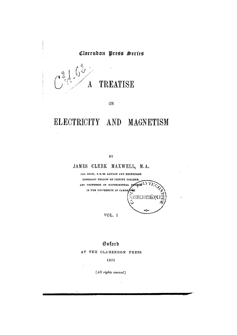
The next step was taken by two self-taught readers of the Treatise. The Englishman Oliver Heaviside, a telegraphist who had left school at 16, and the American Josiah Willard Gibbs, of Yale, abandoned quaternions and each independently created modern vector analysis, with the dot product and the cross product. In 1884 and 1885 Heaviside rewrote Maxwell’s twenty equations as four. That is the form in which they appear in every textbook today.
The four equations
In a vacuum, with charges of density $\rho$ and currents of density $\mathbf J$, the electric field $\mathbf E$ and the magnetic field $\mathbf B$ obey
$$\boxed{\begin{aligned}\nabla\cdot\mathbf E&=\frac{\rho}{\varepsilon_0}\\ \nabla\cdot\mathbf B&=0\\ \nabla\times\mathbf E&=-\frac{\partial\mathbf B}{\partial t}\\ \nabla\times\mathbf B&=\mu_0\mathbf J+\mu_0\varepsilon_0\frac{\partial\mathbf E}{\partial t}\end{aligned}}$$where $\varepsilon_0$ and $\mu_0$ are two constants measured in the laboratory. The divergence $\nabla\cdot$ measures how much a field “flows out” of a point, like water from a spring; the curl $\nabla\times$ measures how much it “swirls” around a point, like water down a plughole. In words:
| Equation | Name | What it says |
|---|---|---|
| 1 | Gauss’s law | Electric field lines begin on positive charges and end on negative ones. |
| 2 | Gauss’s law for magnetism | Magnetic field lines never begin or end: there is no isolated magnetic pole. |
| 3 | Faraday’s law | A changing magnetic field creates an electric field that swirls around it. |
| 4 | Ampère–Maxwell law | A current, or a changing electric field, creates a magnetic field that swirls around it. |
To work out the motion of a charge $q$ with velocity $\mathbf v$, add the Lorentz force, $\mathbf F=q(\mathbf E+\mathbf v\times\mathbf B)$, and all of electromagnetism is there.
A test: Coulomb’s law
The equations contain the old laws. Take a charge $q$ at rest. By symmetry the field points outwards, with the same value $E$ at every point of a sphere of radius $r$. Gauss’s law, in integral form, says that the flux of the field through the sphere is the charge divided by $\varepsilon_0$:
$$E\cdot4\pi r^2=\frac q{\varepsilon_0}\quad\Longrightarrow\quad E=\frac{q}{4\pi\varepsilon_0r^2}.$$This is Coulomb’s law, of 1785: the force falls off with the square of the distance, like Newton’s gravity. The reason is geometric: the same lines of force spread over an area $4\pi r^2$, which grows with the square of the radius.
Exercise: the field E = (−y, x, 0) swirls around the z axis. Calculate its curl and its divergence.
The curl is $\nabla\times\mathbf E=\left(\frac{\partial E_z}{\partial y}-\frac{\partial E_y}{\partial z},\ \frac{\partial E_x}{\partial z}-\frac{\partial E_z}{\partial x},\ \frac{\partial E_y}{\partial x}-\frac{\partial E_x}{\partial y}\right)=(0,0,1-(-1))=(0,0,2)$. The divergence is $\frac{\partial(-y)}{\partial x}+\frac{\partial x}{\partial y}+0=0$. The field swirls without flowing out of anywhere: non-zero curl, zero divergence, like the lines of a magnetic field around a wire.
Exercise: what is the electric field 1 m from a charge of 1 microcoulomb? Use 1/(4πε₀) ≈ 9 × 10⁹.
$E=9\times10^9\cdot\frac{10^{-6}}{1^2}=9{,}000$ volts per metre. At 2 m the field is four times smaller, 2,250 V/m; at 10 m, a hundred times smaller, 90 V/m.
Sources: James Clerk Maxwell, “A dynamical theory of the electromagnetic field”, Philosophical Transactions of the Royal Society 155 (1865) · Michael J. Crowe, A History of Vector Analysis (Dover, 1994), chs. 4–5 · The Feynman Lectures on Physics, volume II, chapter 18.
All topics on James Clerk Maxwell · ← The speeds of molecules: the Maxwell distribution · The displacement current: the missing term →