
Euler's Eyes
2026-10-30
Classical probability and the Gaussian integral
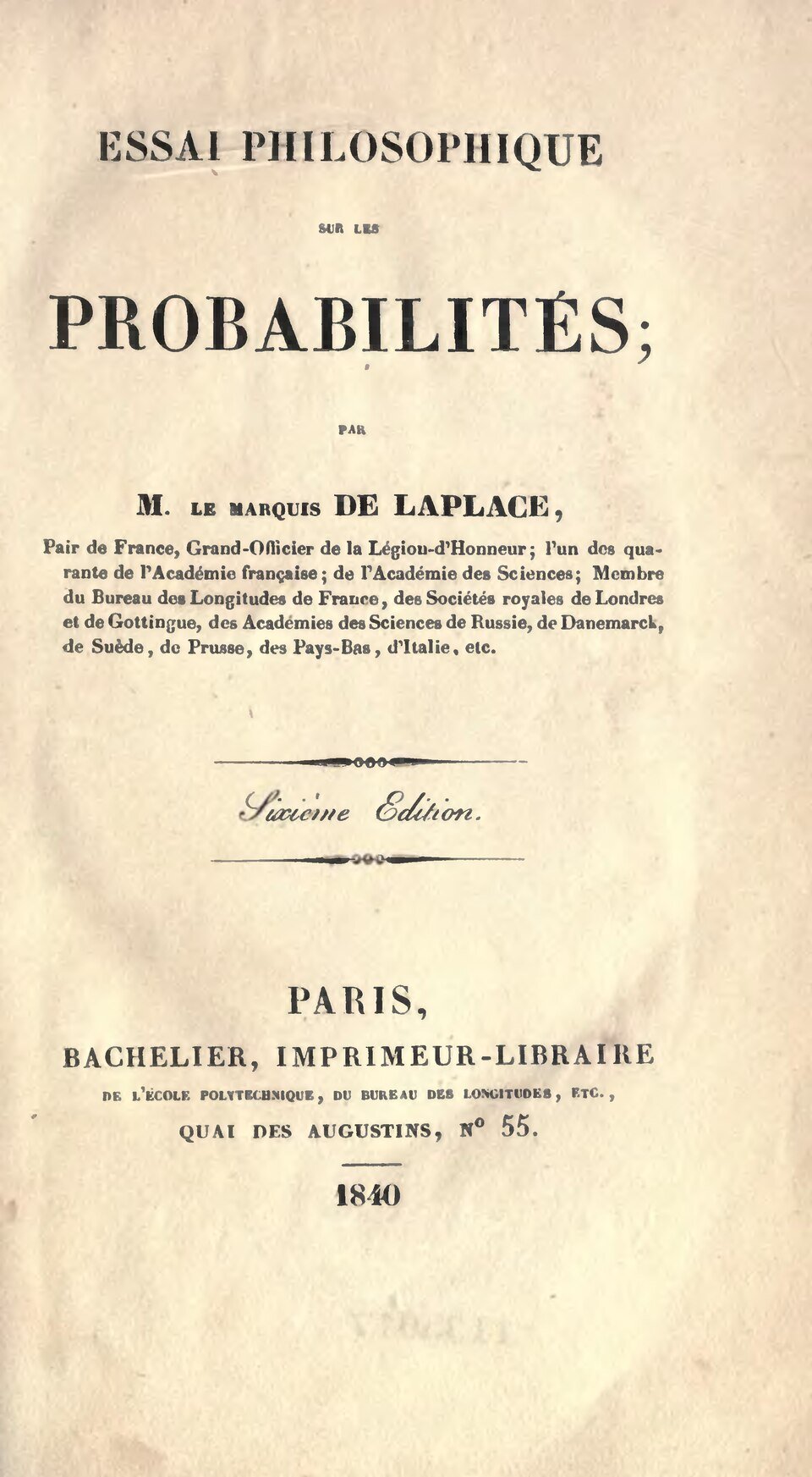
Mathematical probability began with games of chance, in the letters between Pascal and Fermat in 1654, and gained its first great theorem with Jakob Bernoulli’s law of large numbers. Laplace turned it into a complete theory. His first work on the subject dates from 1774; the Analytic Theory of Probabilities, of 1812, gathered almost forty years of research, and the Philosophical Essay on Probabilities, of 1814, explained it all to the public without formulas.
The classical definition
The theory of chance consists in reducing all events of the same kind to a certain number of equally possible cases, that is, such that we are equally undecided about their existence, and in determining the number of cases favourable to the event whose probability is sought.
— Pierre-Simon Laplace, Philosophical Essay on Probabilities (1814)
It is the definition taught at school:
$$P = \frac{\text{number of favourable cases}}{\text{number of possible cases}}.$$The delicate point lies in the words “equally possible”. With two dice there are 11 possible sums, from 2 to 12, but they are not equally likely. The equally possible cases are the 36 pairs (first die, second die). The sum 7 appears in 6 of them, from (1, 6) to (6, 1), and so has probability $\frac{6}{36} = \frac{1}{6}$; the sum 2 appears only in (1, 1), with probability $\frac{1}{36}$.
The integral of e to the minus x squared
While studying sums of many chances, Laplace needed an integral that appears throughout statistics:
$$\int_{-\infty}^{\infty} e^{-x^2}\,dx = \sqrt{\pi}.$$Abraham de Moivre had already used the result in numerical form in 1733; Laplace proved it in 1774. The prettiest proof is a trick: instead of computing the integral $I$, compute $I^2$, which is an integral over the plane:
$$I^2 = \int_{-\infty}^{\infty}\int_{-\infty}^{\infty} e^{-(x^2+y^2)}\,dx\,dy.$$In polar coordinates, $x^2 + y^2 = r^2$ and the area element is $r\,dr\,d\theta$:
$$I^2 = \int_0^{2\pi}\int_0^{\infty} e^{-r^2}\,r\,dr\,d\theta = 2\pi \cdot \left[-\frac{e^{-r^2}}{2}\right]_0^{\infty} = 2\pi \cdot \frac{1}{2} = \pi.$$Hence $I = \sqrt{\pi}$. It is this integral that makes the area under the normal curve come out exactly 1.
Approximating the enormous
Laplace developed a method for estimating integrals of functions with a very tall, narrow peak: near the peak, every such function looks like $e^{-x^2}$. This Laplace’s method gives, for example, Stirling’s formula for the factorial:
$$n! \approx \sqrt{2\pi n}\left(\frac{n}{e}\right)^n.$$For $n = 10$ the formula gives about $3\,598\,696$, against the exact value $3\,628\,800$: an error of 0.8%. And the relative error shrinks as $n$ grows. With approximate factorials, Laplace could compute probabilities involving thousands of cases that nobody could count by hand.
Exercise: a sum of 10 with two dice
What is the probability that the sum of two dice is 10? And that it is at least 10?
Sum 10: (4, 6), (5, 5), (6, 4), three cases out of 36, or $\frac{1}{12}$. Sum 11: (5, 6), (6, 5), two cases. Sum 12: (6, 6), one case. At least 10: $\frac{3 + 2 + 1}{36} = \frac{6}{36} = \frac{1}{6}$.
Exercise: changing the scale
Use $\int_{-\infty}^{\infty} e^{-x^2}\,dx = \sqrt{\pi}$ to compute $\int_{-\infty}^{\infty} e^{-x^2/2}\,dx$.
Set $x = \sqrt{2}\,u$, so that $\frac{x^2}{2} = u^2$ and $dx = \sqrt{2}\,du$:
$$\int_{-\infty}^{\infty} e^{-x^2/2}\,dx = \sqrt{2}\int_{-\infty}^{\infty} e^{-u^2}\,du = \sqrt{2}\sqrt{\pi} = \sqrt{2\pi}.$$That is why the standard normal density has the factor $\frac{1}{\sqrt{2\pi}}$ in front.
Sources: Pierre-Simon Laplace, “Mémoire sur la probabilité des causes par les événements”, Mémoires de mathématique et de physique présentés à l’Académie 6 (1774) · Pierre-Simon Laplace, Théorie analytique des probabilités (1812) · Pierre-Simon Laplace, Essai philosophique sur les probabilités (1814) · Stephen M. Stigler, The History of Statistics (1986) · Anders Hald, A History of Mathematical Statistics from 1750 to 1930 (1998).
All topics on Pierre-Simon Laplace · ← Laplace’s expansion of determinants · The central limit theorem →