
Euler's Eyes
2026-10-14
The Analytical Mechanics: a book without figures
Open Newton’s Principia of 1687 and you will see figures on almost every page: triangles, ellipses, arrows, tangents. Open Lagrange’s Analytical Mechanics, published a century later in 1788, and you will see none. The author warns of this himself in the preface, with pride, and adds:
Those who love analysis will be pleased to see mechanics become a new branch of it, and will be grateful to me for having thus extended its domain.
— Joseph-Louis Lagrange, preface to the Analytical Mechanics (1788)
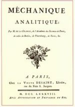
The book was written in Berlin and brought to Paris almost finished. No publisher wanted to risk money on such a difficult treatise, and it was the young Adrien-Marie Legendre who persuaded a bookseller to publish it and corrected the proofs. It is said that when the printed volume arrived, Lagrange went two years without opening it, during one of his periods of depression.
The trouble with forces
In Newton’s mechanics, to know how a body moves you must list all the forces acting on it and add them like arrows. In a pendulum, for example, the weight and the tension of the string act. The weight is easy; the tension is not: it changes at every instant and nobody knows it in advance. It serves only to keep the bob attached to the string, and even so it has to be calculated before you get to the motion.
Lagrange wanted a method in which these constraint forces simply did not appear.
One function for everything
Lagrange’s idea was to describe the system by coordinates chosen at will, whichever are most natural. For the pendulum one number is enough: the angle $\theta$ of the string from the vertical. Then you write two energies in terms of these coordinates:
- $T$, the energy of motion (today called kinetic energy);
- $V$, the energy stored by position (today, potential energy).
And you form a single function, which today is called the Lagrangian:
$$L=T-V.$$The true motion is the one that satisfies the Euler–Lagrange equation, now with time $t$ in place of $x$:
$$\frac{d}{dt}\frac{\partial L}{\partial\dot q}-\frac{\partial L}{\partial q}=0,$$where $q$ is the coordinate and $\dot q$, with a dot on top, is its velocity, in Newton’s notation. It is a recipe: write $L$, differentiate, set equal to zero. There are no figures and no arrows.
First test: free fall
For a body of mass $m$ at height $h$, the energy of motion is $T=\frac12m\dot h^2$ and the stored energy is $V=mgh$. So
$$\begin{aligned}L&=\tfrac12m\dot h^2-mgh,\\ \frac{\partial L}{\partial\dot h}&=m\dot h,\qquad\frac{\partial L}{\partial h}=-mg.\end{aligned}$$The equation becomes $m\ddot h+mg=0$, or $\ddot h=-g$: the body falls with constant acceleration $g$. It is Galileo’s law, recovered without drawing a single arrow.
The pendulum
Now the example where Newton struggles. A bob of mass $m$ hangs from a string of length $\ell$. With angle $\theta$, the bob moves with speed $\ell\dot\theta$ and sits at a height $-\ell\cos\theta$ below the point of suspension. So
$$L=\tfrac12m\ell^2\dot\theta^2+mg\ell\cos\theta.$$Differentiating, $\frac{\partial L}{\partial\dot\theta}=m\ell^2\dot\theta$ and $\frac{\partial L}{\partial\theta}=-mg\ell\sin\theta$. Lagrange’s equation gives
$$\begin{aligned}&m\ell^2\ddot\theta+mg\ell\sin\theta=0\\ &\Longrightarrow\quad\ddot\theta=-\frac g\ell\sin\theta.\end{aligned}$$The tension of the string never appeared. By choosing $\theta$ as the coordinate, the string is already “inside” the description: the bob has no way of leaving the circle. For small angles, $\sin\theta\approx\theta$ and the equation becomes that of the spring, with period
$$P=2\pi\sqrt{\frac\ell g}.$$A scientific poem
The method works for systems with any number of coordinates: double pendulums, spinning tops, planets, vibrating strings. In 1834 the Irishman William Rowan Hamilton rewrote Lagrange’s equations in an even more symmetrical form and wrote of the book:
Lagrange has perhaps done more than any other analyst to give extent and harmony to such deductive researches […]. He has made of his great work on the Mécanique Analytique a kind of scientific poem.
— William Rowan Hamilton, On a General Method in Dynamics (1834)
Exercise: what length of pendulum has a period of 2 seconds?
From $P=2\pi\sqrt{\ell/g}$, we have $\ell=g\left(\frac{P}{2\pi}\right)^2=9.81\cdot\frac1{\pi^2}\approx0.994$ m. This is the seconds pendulum: each swing takes 1 second. In 1791 the metric commission, of which Lagrange was a member, discussed using this length as the definition of the metre. It preferred one ten-millionth of the quarter meridian of the Earth, because $g$ changes from place to place.
Exercise: the spring by Lagrange's recipe
A mass $m$ on a spring of constant $k$, displaced by $x$, has $T=\frac12m\dot x^2$ and $V=\frac12kx^2$. Then $L=\frac12m\dot x^2-\frac12kx^2$, $\frac{\partial L}{\partial\dot x}=m\dot x$ and $\frac{\partial L}{\partial x}=-kx$. The equation gives $m\ddot x+kx=0$, the same one obtained from Hooke’s law and $F=ma$.
Sources: Joseph-Louis Lagrange, Méchanique analitique (1788), on the Internet Archive · biography of Lagrange, MacTutor · William Rowan Hamilton, “On a General Method in Dynamics”, Philosophical Transactions (1834).
All Lagrange topics · ← The calculus of variations: a letter from a 19-year-old · The Lagrange points: where gravity balances →