
Euler's Eyes
2026-10-10
Gaussian quadrature: integrate with two points
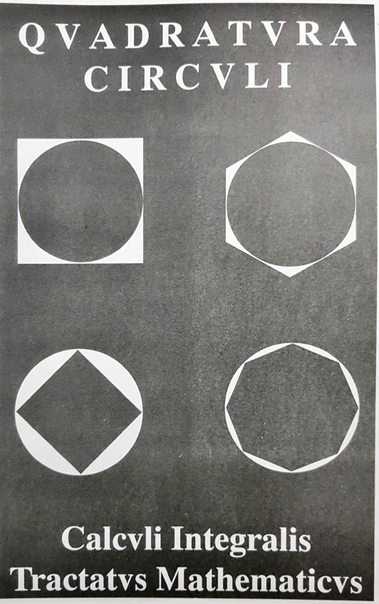
“Squaring” is the old name for calculating an area. The Greeks approximated the area of the circle by polygons with increasingly more sides, and integral calculus was born. The practical problem is: how to calculate the area under a curve doing few math?
The simplest way is the trapezoid rule: look at the curve only at the ends, $x = -1$ and $x = 1$, and calculate the area of the trapezoid. In 1814, Gauss asked: What if I can choose where to look? With two points $\pm t$ and weights equal to 1, the estimate is
He wanted the formula to match exactly as many polynomials as possible:
Finding the Gaussian point (click to advance)
- For $f(x) = 1$: the area is 2, and the formula gives $1 + 1 = 2$. ✓ Works for any $t$.
- For $f(x) = x$ (and $x^3$): the area is 0, and the formula gives $-t + t = 0$. ✓ It also works every time.
- For $f(x) = x^2$: the area is $\frac{2}{3}$, and the formula gives $t^2 + t^2 = 2t^2$.
- Equating: $2t^2 = \frac{2}{3}$, then $t^2 = \frac{1}{3}$ and $t = \frac{1}{\sqrt{3}} \approx 0{,}577$.
- Result: with just two points, the rule hits spotly any polynomial of degree up to 3.
Today this method is called Gauss-Legendre quadrature and is found in almost every program that calculates integrals. This is what allows you to find areas under curves, lengths and volumes graphically and visual, adding little pieces.
All topics by Carl Friedrich Gauss · ← Systems of equations: the determinant and Gaussian elimination · Other contributions and legacy →